At the end of this reading, you should be able to interpret followings:

• Enhanced Regressor Modelling
• PyTorch ML Model-Method Architecture
• Neural Network Layerings {Input > Hidden (Linear Transformation, Batch Normalization, GELU Activation, Dropout) > Output with Sigmoid Activation}
• Model Definition and Forward Propagation in Machine Learning

📌 Introduction:

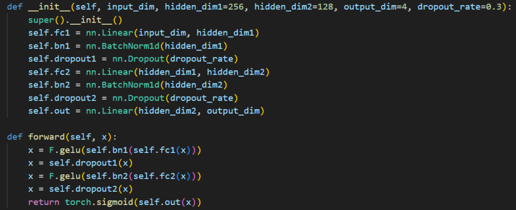
Machine Learning models are often perceived as black boxes, especially when implemented using Deep Learning Frameworks like PyTorch. This article aims to demystify a Supervised Multi-label Variables Classification Model (these variables can be psycho-cognito aspects of a language piece or video or image etc.) built using PyTorch by explaining the Model-Method Paradigm. Below in black screen is the ‘Code snippet copy of a PyTorch Model’ we are going to decode in simple human language.

In PyTorch, a custom model is usually defined by inheriting from nn.Module class. This class includes:

• Model Definition (__init__) : where the architecture is built.
• Forward Method (forward) : where how data flows through the model is defined.

Above code snippet is core of a “Enhanced Variables Regressor” Supervised ML Model; here the term “Variables” remains contextual to your needs and objective. I’ll walk you through this code line-by-line further to capture the logic, flow, and design rationale behind each line of this code. We’ll discover how to interpret the architecture and make it production-ready by building a prediction pipeline and visualizing variable probabilities. Whether you’re a curious student or a working data scientist, this explanation will equip you with the understanding needed to dissect, adapt, or extend similar models in your own Supervised ML projects.

However you shall require to define the before and after steps of the core central model; before steps like preparing your raw training data, preprocessing that data and data features engineering. In after steps you shall require to evaulate your output through test data. So in a way we intend to talk in this article specifically about the core ML Model and Method of complete pipeline. I shall be covering these before and after steps in another dedicated article, because covering complete pipline in one article shall make it out of context bigger than what our aim is to achieve through this article. So we proceed for understanding the core architecture of the code snippet given above as next section of this article below.

---

🏗️ Code Architecture

As said above a typical Supervised Machine Learning Model usually composes of a Model and a Method blocks.

🔹 1. Model – Structure Definition (__init__) : This section defines the architecture – layers, normalization, and dropout. Here below is the line-by-line decoding of Model code:

1. def __init__(self, input_dim, hidden_dim1=256, hidden_dim2=128, output_dim=4, dropout_rate=0.3) : def __init__ is the model definition constructor where model layers with regulations are defined in parenthesis (self, …..). The regulations defined in parameters take in:
   • self: It is a placeholder for the object it is placed in/with. Like any other convention, tt tells Python that the variables belong to the current object instance and must be the first parameter of instance method(s).
   • input_dim: Size of input features (e.g., embedding or TF-IDF vector). It comes from the trained and preprocessed data (as said above I shall write this part in another article).
   • hidden_dim1: Number of units in the 1st hidden layer (default: 256).
   • hidden_dim2: Units in 2nd hidden layer (default: 128).
   • output_dim: Number of output values (e.g., 4 variables related to psycho-cognito aspect of a language piece or video or image).
   • dropout_rate: Fraction of units to drop (default: 0.3).
2. super().__init__(): It calls the constructor of the parent class (nn.Module) to properly initialize the Neural Network Model.
3. self.fc1 = nn.Linear(input_dim, hidden_dim1): The first fully connected i.e. fc dense layer (input → 256) by taking input of size input_dim and maps it to a hidden layer with hidden_dim1 neurons. Its function is to learn weighted combinations of features.
4. self.bn1 = nn.BatchNorm1d(hidden_dim1): bn1 applies Batch Normalization i.e. bn for first layer. This helps in stabilizing and speeding up training by normalizing activations across the batch.
5. self.dropout1 = nn.Dropout(dropout_rate): Dropout1 applies dropout after the first hidden layer activation. It randomly zeroes out a fraction (dropout_rate) of neurons during training for regularization. It prevents overfitting by randomly disabling neurons.
6. self.fc2 = nn.Linear(hidden_dim1, hidden_dim2): fc2 is second fully connected layer (256 → 128), transforming from hidden_dim1 to hidden_dim2.
7. self.bn2 = nn.BatchNorm1d(hidden_dim2): bn2 applies Batch Normalization after the second layer.
8. self.dropout2 = nn.Dropout(dropout_rate): dropout2 applies Dropout after second hidden layer activation for further regularization.
9. self.out = nn.Linear(hidden_dim2, output_dim): out defines the final linear output layer (128 → 4 variable scores). It maps the second hidden layer to the output_dim size, typically representing class scores or prediction target.

So the Model Architecture defines Layer sizes, Dropout regulations and Batch Normalization. And these are stored in the object (self.fc1, self.dropout1 etc.), ready to be used in the forward() method, explained next.

---

🔹 2. Method – Forward Propagation (forward): This part describes how data flows through the model during training and inference. Let’s understand its coding and functioning both:

1. def forward(self, x): It defines how the data moves through the model during inference or training.
2. x = F.gelu(self.bn1(self.fc1(x))): It passes the input x through fc1, bn1 and F.gelu. GELU Activation here smoothens and makes noise-robust function well-suited to language (NLP) data.
3. x = self.dropout1(x): It applies the dropout after the first hidden transformation.
4. x = F.gelu(self.bn2(self.fc2(x))): Serves same function as hidden layer 1.
5. x = self.dropout2(x): It applies the dropout after the second hidden transformation.
6. return torch.sigmoid(self.out(x)): It passes data through the final layer to get output_dim logits by applying sigmoid activation to squash outputs between 0 and 1. As ours is a multi-label classification model so sigmoid outputs independent probabilities for each variable class.

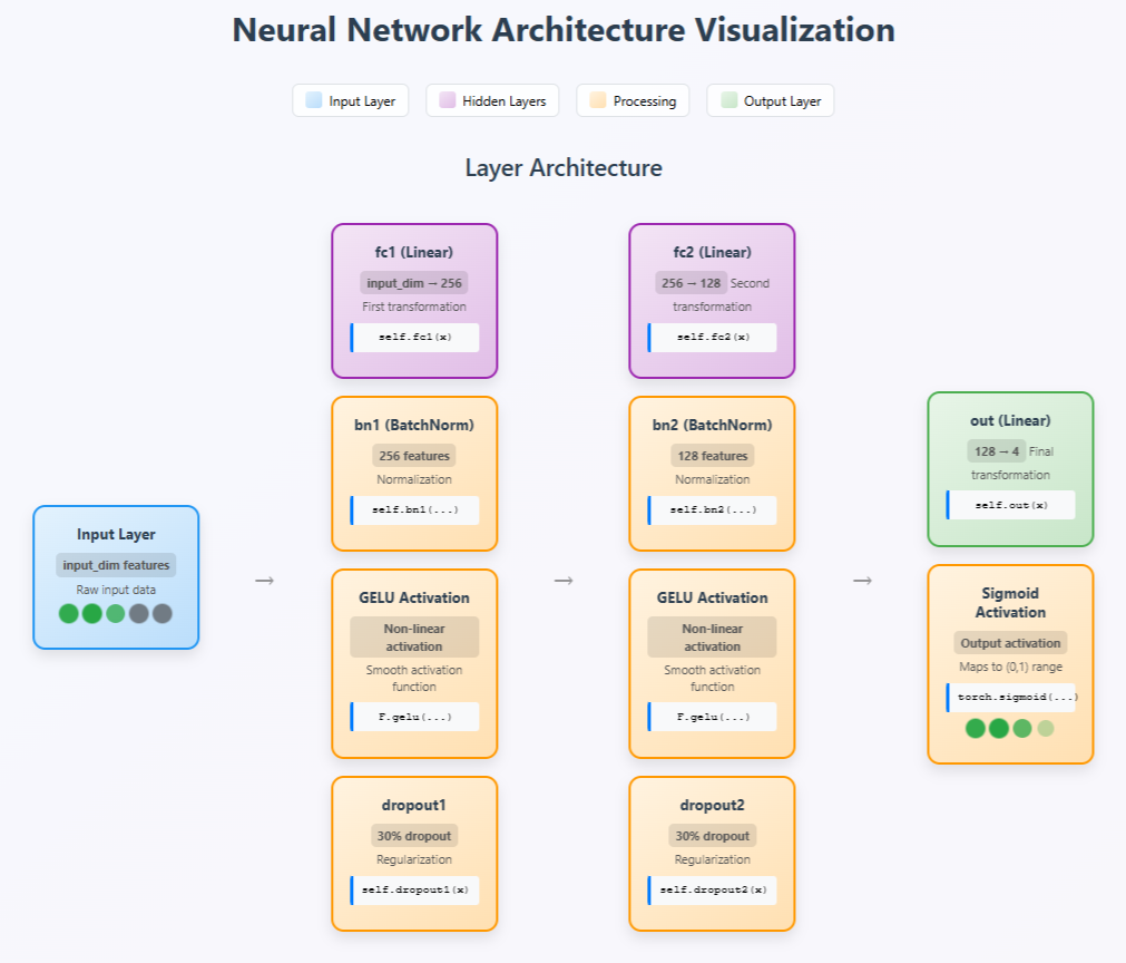
Neural Network Architecture Visualization

What we have tried to interpret from above reading is depicted in below image. While in above explanations, we understood each code line individually, here below inforgraphic present these code layering in conjucture with each other. It gives the reflection of complete steps interacting with each other. So as a customory norm of any NN Model Architecture, this visualization also presents the three standard layers of our model viz-a-viz Input Layer, Hidden Layer and Output Layer. Hiddern layer is consisted of two vertical column having fc1 and fc2 at the top and then their correspoding Batch Normalization, GELU Activation and Dropouts. Output Layer is supported through Sigmoid Activation. 

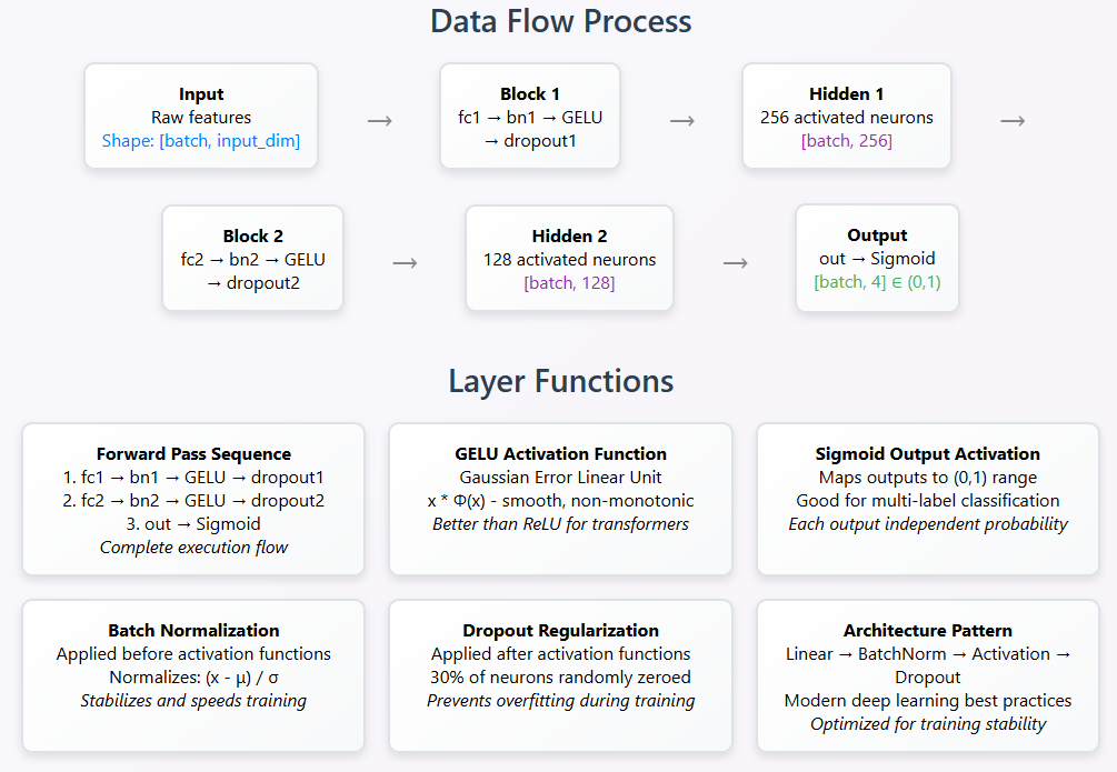
Step-by-step explanation of Model-Method in sequential conjunction

What all layers and each constituent of each layer does what is presented for you in below inforgraphic consisted of “Data Layer Process Pipeline” and Layer Functions. Combined both Model-Method forms a Multi-Layer Perceptron which takes numerical/text feature vector (e.g. TF-IDF or embeddings) as input; classifies them into one or more variable categories which can further be used with SoftMax for single-label or sigmoid for multi-label as shown below:

• fc1 → bn1 → GELU → dropout1: First transformation with activation and regularization.
• fc2 → bn2 → GELU → dropout2: Second transformation.
• out → sigmoid: Produces 4 normalized output probabilities between 0 and 1.

In a nutshell, what we interpreted above can also be termed as “Deep FeedForward Neutral Network designed for multi-label variables classification.

💡 Why Model-Method Structure?: PyTorch encourages clean modular design:

• __init__() allows you to declare and manage all trainable layers.
• forward() is where you define the logic of computation.

This separation improves readability, reusability, and makes debugging easier.

🔗 Building a Prediction Pipeline: To make this model production-ready:

1. Preprocess text into numerical form (e.g., TF-IDF or BERT embeddings).
2. Load the trained model.
3. Predict contextual variables such as pscyho-cognito aspects of a language piece.

✅ Capabilities

• It can be used for doing the cognitive, intent, sentiment and psychological analysis of a text transcript or group of text transcripts. Here be attentive that this code is just of the ML model core ready to accept the trained data as input (for supervised or semi-supervised machine learning architecture) and then forwarded to accept test inputs to testify. I shall write a separate article on training data and testifying data parts a separate article.
• Supports text classification tasks like search or health intent prediction.
• Easily integrable into PyTorch-based pipelines.
• Generalizable to other domains with similar multi-label needs.

⚠️ Limitations

• Input must be vectorized (e.g., using TF-IDF or transformers).
• May underperform on complex linguistic tasks unless combined with contextual embeddings.
• Doesn’t handle sequences; for that, models like RNNs or transformers are better.

🧾 Conclusion: The Enhanced Regressor Model presented above is a supervised, feedforward neural network tailored for multi-label variables classification tasks in NLP. Its design leverages:

• Deep fully connected layers,
• GELU activations for smooth learning,
• Batch normalization and dropout for regularization,
• Sigmoid output for multi-label prediction.

📚 References

• Hendrycks & Gimpel (2016) on GELU: https://arxiv.org/abs/1606.08415
• Ioffe & Szegedy (2015) on BatchNorm: https://arxiv.org/abs/1502.03167
• PyTorch Documentation: https://docs.pytorch.org/docs/stable/nn.html
• GELU (Gaussian Error Linear Unit): A mathematical Activation function used in fundamental building blocks of neural networks which provides more nuanced activation patterns, used in modern popular architectures like BERT, GPT. GELU in our model is used in the hidden layers internal processing which allows network to learn complex, non-linear patterns with smooth gradients.
• Sigmoid Function maps any real number to (0,1) range in S-shaped curve to do smooth transition and does the probabilistic interpretation of the output. It is used for output formatting for a perfect multi-label classification with probabilities for each class. However it has been of logistic regression class but now used for probability outputs like in our model.